library(tidyverse)
library(rgbif)
library(gpx)California Pitcher Plant
species distribution
GIS
maps
data
trail run
exercise
explore
cobra lily
illustration
–Cobra Lily (Darlingtonia californica)
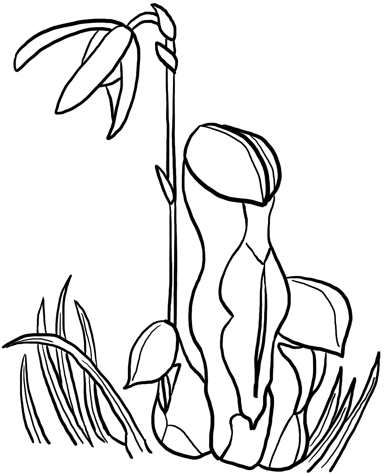
Spring is in full swing in the higher elevations around Mount Shasta and the surrounding ranges. I am always struck by the large patches of Cobra Lilies that grow along nutrient poor seeps in alpine meadows. I nearly always stop to take some photos and take in all the cool colors and shapes when out on training runs or hikes. I have made many observations of these over the past few years, but here is a quick post to pull out observations from GBIF.
Load the libraries.
Make the large Northern California polygon to look for observations in GBIF.
norcal_geometry <- paste('POLYGON((-124.4323 42.0021, -121.5045 42.0021, -121.5045 40.194, -124.4323 40.194, -124.4323 42.0021))')

cobra_lily <- occ_data(scientificName = "darlingtonia californica", hasCoordinate = TRUE, limit = 1000,
                   geometry = norcal_geometry)
head(cobra_lily)
$meta
$meta$offset
[1] 900
$meta$limit
[1] 100
$meta$endOfRecords
[1] FALSE
$meta$count
[1] 1582
$data
# A tibble: 1,000 × 128
key scien…¹ decim…² decim…³ issues datas…⁴ publi…⁵ insta…⁶ hosti…⁷ publi…⁸
<chr> <chr> <dbl> <dbl> <chr> <chr> <chr> <chr> <chr> <chr>
1 45123… Darlin… 41.7 -124. cdc,c… 50c950… 28eb1a… 997448… 28eb1a… US
2 45163… Darlin… 41.9 -124. cdc,c… 50c950… 28eb1a… 997448… 28eb1a… US
3 45191… Darlin… 41.9 -124. cdc,c… 50c950… 28eb1a… 997448… 28eb1a… US
4 45253… Darlin… 41.9 -124. cdc,c… 50c950… 28eb1a… 997448… 28eb1a… US
5 45280… Darlin… 41.7 -124. cdc,c… 50c950… 28eb1a… 997448… 28eb1a… US
6 40286… Darlin… 41.9 -124. cdc,c… 50c950… 28eb1a… 997448… 28eb1a… US
7 40347… Darlin… 40.7 -124. cdc,c… 50c950… 28eb1a… 997448… 28eb1a… US
8 40394… Darlin… 41.6 -124. cdc,c… 50c950… 28eb1a… 997448… 28eb1a… US
9 41655… Darlin… 41.8 -124. cdc,c… 50c950… 28eb1a… 997448… 28eb1a… US
10 40629… Darlin… 41.9 -124. cdc,c… 50c950… 28eb1a… 997448… 28eb1a… US
# … with 990 more rows, 118 more variables: protocol <chr>, lastCrawled <chr>,
# lastParsed <chr>, crawlId <int>, basisOfRecord <chr>,
# occurrenceStatus <chr>, taxonKey <int>, kingdomKey <int>, phylumKey <int>,
# classKey <int>, orderKey <int>, familyKey <int>, genusKey <int>,
# speciesKey <int>, acceptedTaxonKey <int>, acceptedScientificName <chr>,
# kingdom <chr>, phylum <chr>, order <chr>, family <chr>, genus <chr>,
# species <chr>, genericName <chr>, specificEpithet <chr>, taxonRank <chr>, …Quick map of observations.
cobra_lily_coords <- cobra_lily$data[ , c("decimalLongitude", "decimalLatitude", "occurrenceStatus", "coordinateUncertaintyInMeters", "institutionCode", "references")]

maps::map(database = "state", region = "california")
points(cobra_lily_coords[ , c("decimalLongitude", "decimalLatitude")], pch = ".", col = "red", cex = 3)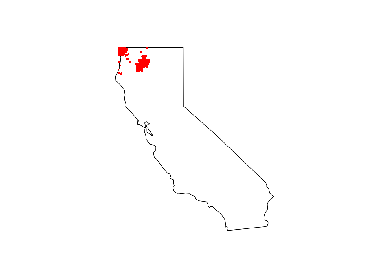
Pull in my run data using the gpx R library and subset the route to make plotting easier.
run <-  read_gpx('~/DATA/data/cobra_lily_run.gpx')
TrailRun1 <- as.data.frame(run$routes)
Make a quick run plot.
TrailRun_plot <- ggplot() +
          geom_point(data = TrailRun1, aes(x = Longitude, y = Latitude), color = 'black') +
          xlab("Longitude") + ylab("Latitude")
TrailRun_plot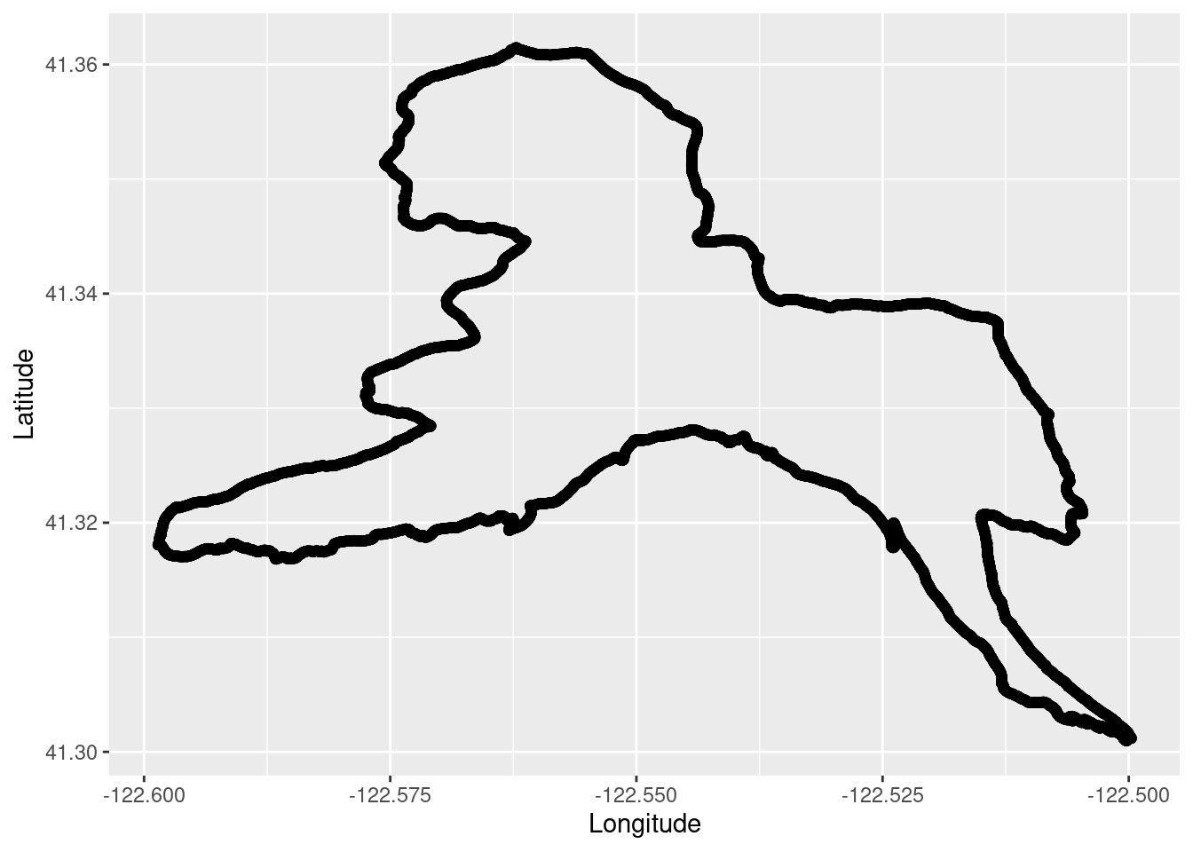
Subset the larger California dataset to only include a zoomed in portion where I ran based on the maximum and minimum coordinates from the run plot above.
cobra_lily_coords_sub <- subset(cobra_lily_coords, decimalLatitude > 41.3 & decimalLatitude < 41.365 & decimalLongitude > -122.6 & decimalLongitude < -122.5 )Overlay the plots and add a triangle for the seep where I observed some Cobra Lilies next to the trail.
TrailRun_plot2 <- ggplot() +
          coord_quickmap() +
          geom_point(data = TrailRun1, aes(x = Longitude, y = Latitude), color = 'black') +
          geom_point(data=cobra_lily_coords_sub, aes(x = decimalLongitude, y = decimalLatitude), color = 'red') +
          geom_point(aes(x = -122.55, y = 41.325), pch=25, size= 12, colour="purple") +
          xlab("Longitude") + ylab("Latitude")
TrailRun_plot2
In a follow-up post we will import some additional environmental data to make a multi-layered map.