Cody Markelz - Edward Stuhl Wildflowers

I have been working on identifying and painting various local wildflowers from the book Mount Shasta Wild Flowers A Field Guide featuring the water color paintings of Edward Stuhl. Stuhl was an artist and mountaineer that gradually painted 189 plants over a 50 year career exploring the greater Mount Shasta area. All of his paintings are available to view online at CSU Chico here. I was interested in what sort of publicly available observation data there was for some of the more rare species. I downloaded the original list here, and made a few quick formatting edits to get it ready to pull into R.

Load the libraries.

library(tidyverse)
library(readxl)
library(rgbif)
library(data.table)

Pull in the data, take a quick look, and make a character vector of the species names for the GBIF query.

shasta_plants <- read_excel("~/DATA/data/mount.shasta.plant.list.edit.xlsx")

head(shasta_plants)

# A tibble: 6 × 5
  ID           Family           Genus       species    `subspecies or variety`
  <chr>        <chr>            <chr>       <chr>      <chr>                  
1 Ferns_Allies Dennstaedtiaceae Pteridium   aquilinum  var. pubescens         
2 Ferns_Allies Dryopteridaceae  Polystichum scopulinum <NA>                   
3 Ferns_Allies Equisetaceae     Equisetum   arvense    <NA>                   
4 Ferns_Allies Equisetaceae     Equisetum   hyemale    ssp. affine            
5 Ferns_Allies Ophioglossaceae  Botrychium  pinnatum   <NA>                   
6 Ferns_Allies Ophioglossaceae  Botrychium  pumicola   <NA>

dim(shasta_plants)

[1] 482   5

shasta_plants$query <- as.character(paste(shasta_plants$Genus, shasta_plants$species))
shasta_species <- shasta_plants$query
head(shasta_species)

[1] "Pteridium aquilinum"    "Polystichum scopulinum" "Equisetum arvense"     
[4] "Equisetum hyemale"      "Botrychium pinnatum"    "Botrychium pumicola"

Make a polygon to query from within and run a GBIF query iterating through the shasta_species character vector. The query takes a while for building this webpage, so I am going to just load the result instead to list the objects. If you want to run the query uncomment the following few lines.

mt_shasta_geometry <- paste('POLYGON((-122.600528 41.551515, -122.001773 41.551515, -122.001773 41.252791, -122.600528 41.252791, -122.600528 41.551515))')

# shasta_all <- occ_data(scientificName = shasta_species, hasCoordinate = TRUE, limit = 100,
#                   geometry = mt_shasta_geometry)

load("~/DATA/data/Stuhl_Shasta_species_GBIF.RData")
ls()

[1] "mt_shasta_geometry" "shasta_all"         "shasta_plants"     
[4] "shasta_species"

Iterate through the GBIF query list and pull out the latitude and longitude of each observation and bind them all together.

shasta_species_coords_list <- vector("list", length(shasta_species))
names(shasta_species_coords_list) <- shasta_species

for (x in shasta_species) {
  coords <- shasta_all[[x]]$data[ , c("decimalLongitude", "decimalLatitude", "occurrenceStatus")]
  shasta_species_coords_list[[x]] <- data.frame(cbind(species = x, coords))
}

species_coord_df <- rbindlist(shasta_species_coords_list, fill = T)
head(species_coord_df)

               species decimalLongitude decimalLatitude occurrenceStatus
1: Pteridium aquilinum        -122.3233        41.28727          PRESENT
2: Pteridium aquilinum        -122.3304        41.31041          PRESENT
3: Pteridium aquilinum        -122.0664        41.27251          PRESENT
4: Pteridium aquilinum        -122.0780        41.28300          PRESENT
5: Pteridium aquilinum        -122.3066        41.27987          PRESENT
6: Pteridium aquilinum        -122.4471        41.44342          PRESENT

Make a quick plot of the data removing the legend or it will overwhelm the plot with the large number of species.

species_p1  <- ggplot(species_coord_df, aes(x=decimalLongitude, y = decimalLatitude, color = species)) +
                geom_point() +
                labs(x = "Longitude", y = "Latitude", title = "Mount Shasta Plant Species Observations") + theme(legend.position="none")
species_p1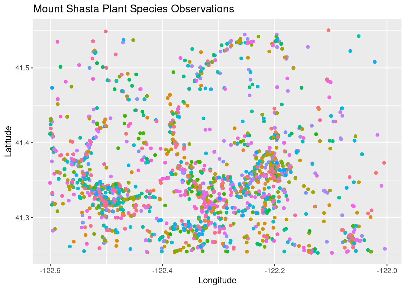

ggsave("~/DATA/images/stuhl_species.png")

A lifetime of exploration just in my general area! I hope to share more paintings of the same species as I am out and about around Mount Shasta.